Introduction
Earlier in the year I wrote about how the objective function of an optimization problem is decomposed and partially evaluated so an algorithm that uses that function runs faster. I found this technique so interesting that I tried to explain it in that post. But the goal wasn’t to just understand the decomposing of an objective function. I needed to design a fast algorithm to solve the $\alpha$-neighbor $p$-center problem (ANPCP), as I mentioned in the other post, and while researching to do so, I came across the concept of the fast interchange or fast swap and how it was applied to other location problems (not the ANPCP). I also wrote about it in that post, however, at that moment I didn’t have a working algorithm for the problem, and I just noticed that I didn’t include some definitions there like that of heuristic, so:
A heuristic is any approach to problem solving that employs a practical method that is not guaranteed to be optimal, perfect, or rational, but is nevertheless sufficient for reaching an immediate, short-term goal or approximation.
In that post, I concluded that I would have to do “manual” tests to see where exactly the adapted algorithm was failing… ok boomer.
Although careful experiments were needed to detect the errors, I thought that recurring to pen and paper was too much.
I ended up preferring Gen-Z cutting-edge futuristic technologies instead and tested the algorithm in Jupyter Notebooks (/s) using small instances of the ANPCP.
After four notebooks of testing and modifying the algorithm, it could finally solve the problem for any $\alpha < p$.
You can check them out here, they are the ones whose filenames start with ieval_, but only the introduction and conclusion explain something, I didn’t document much the whole evaluation process.
The final version of the algorithm was baptized as the Alpha Fast Vertex Substitution (A-FVS) local search heuristic, because it considers the $\alpha$th closest center, it is fast, and it substitutes one vertex for another.
Since then, I have been able to write most of the thesis (big shout-out to my mentor and my revisors!), which I think is more understandable than the previous post, so here is the chapter that reviews the background of the fast interchange concept and explains the observations that led us to the birth of the A-FVS.
Still, I recommend reading that post here before reading this one because there’s relevant context in there. Also, if this post gets too technical and I forgot to explain something or it’s difficult to understand, please let me know via LinkedIn or Twitter and I’ll edit this post 👍.
To the best of our knowledge, implementing a fast interchange local search heuristic to solve the ANPCP hadn’t been considered before. The A-FVS has shown significant speedups of computational time in every test, being around 100 times faster than a simple interchange algorithm, depending on the size of the problem. This shows the power of using the appropriate data structures to improve the runtime of an algorithm.
I’ve been coding this in Python in this repository. I warn you, there’s a high technical debt there and it’s not the cleanest code that I’ve written. But until I refactor it, it is what it is.
The process
A solution to the ANPCP can be improved by applying a local search heuristic, i.e., modifying one or more components of the solution based on some rule, looking for a better objective function value among the space of candidate solutions or neighborhoods, until a local optimum is reached.
A well-known local search procedure is the vertex substitution method, also known as the greedy interchange or swap. This method consists of replacing one of the facilities in the solution, denoted as $f_r$, for another one outside the solution, denoted as $f_i$. The procedure is repeated until no more improvements are found (local optimum reached).
A straightforward local search algorithm was first implemented for the ANPCP, identified as Naive Interchange (NI). This algorithm simply iterates over the set of open facilities and, for each of them, iterates the set of closed facilities. At each iteration, it temporarily removes the current open facility, adds the closed facility, and recalculates the objective function value.
This procedure does $O(p^2mn)$ operations, resulting in inefficient performance, based on preliminary experiments. For this reason, we propose a faster vertex substitution algorithm to obtain solutions faster.
Fast Algorithm for the Greedy Interchange (FAGI)
The fast algorithm for the greedy interchange (FAGI) was first proposed for the $p$-median problem (PMP) by Whitaker (1983)1. The key aspect of this implementation is its ability to find the most profitable candidate facility for removal ($f_r$), given a certain candidate facility for insertion ($f_i$), while partially evaluating the objective function.
What makes this procedure fast is the observation that the profit that would result from applying a swap can be decomposed into two components.
The first one, called gain, identifies the users who would benefit from the insertion of $f_i$ into the solution because each user is closer to it than its current closest facility. The second component, netloss, accounts for all other users that would not benefit from the insertion of $f_i$. If $f_r$ is the current closest facility of a user, then it would have to be reassigned either to its second closest one or to $f_i$, whichever is the closest. In both cases, the cost of serving that user will either increase or remain constant.
These two components are useful as they work as auxiliary data structures that make the algorithm fast, which has a worst-case time complexity of $O(mn)$.
The FAGI was implemented and tested for the ANPCP. Even though this algorithm uses the objective function of the PMP, no solutions were obtained successfully (the algorithm was getting stuck when $\alpha \ge 2$, even with small instances). After analyzing how the algorithm was taking decisions and updating the auxiliary data structures, we observed some key differences between the PMP and the ANPCP which were later crucial to propose an improved adaptation that could obtain solutions for any value of $\alpha$ (where $\alpha < p$).
In the PMP, as well as in the PCP, users are assigned to their closest open facility. Although their objective functions are evaluated differently, in both problems the centers have the same definition. Nonetheless, the definition of a center changes for the ANPCP, because users are assigned not to their closest open facility but their $\alpha$th closest open facility, meaning that there are $\alpha - 1$ open facilities that are closer to any user $u$ than its center.
More formally, let $\phi_k(u)$ be the $k$th closest open facility of any user $u$,
$$ \begin{equation} \phi_\alpha(u) \text{ is determined by all } { \phi_k(u) \mid 1 \le k < \alpha } \end{equation} $$
If for $u$, one of the open facilities closer than its current center is considered to be $f_r$, then this center would no longer be the $\alpha$th closest open facility. Hence, the new center of $u$ denoted as $\phi_\alpha'(u)$ would, by definition, be moved to the next farther open facility, which would be the current $\phi_{\alpha + 1}(u)$.
A visual representation is shown below, where $f_r$ is the gray facility (the one that will be removed from the solution), the black straight line is the assignment of $u$ to its center, and the red line and outline indicate which node will be the new center of $u$ after removing $f_r$.
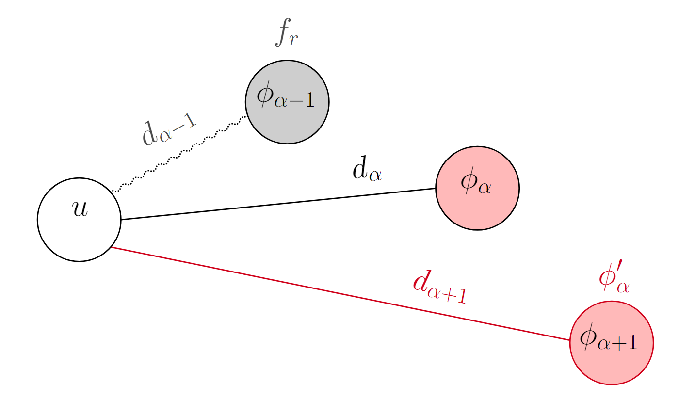
Resulting new center of $u$, $\phi_\alpha'(u)$, after removing its current center $\phi_\alpha(u)$.
“Attraction” here refers to when $f_i$ is closer to $u$ than its center.
The fact that $u$ is attracted to $f_i$ does not necessarily mean that $f_i$ is going to be its new center: it depends on how close $f_i$ is from $u$. This is represented visually in the two figures below. The light red nodes are open facilities, and the dotted lines represent the distances from $u$ to the open facilities that are closer than its center.
Mathematically, let $d_k(u) = d(u, \phi_k(u))$ and $d_i(u) = d(u, f_i)$, then
$$ \begin{equation} \phi_\alpha'(u) \gets \begin{cases} f_i, & \text{if } d_{\alpha - 1}(u) < d_i(u) < d_\alpha(u) \\ \phi_{\alpha - 1}(u), & \text{if } d_i(u) < d_{\alpha - 1}(u) \end{cases} \end{equation} $$
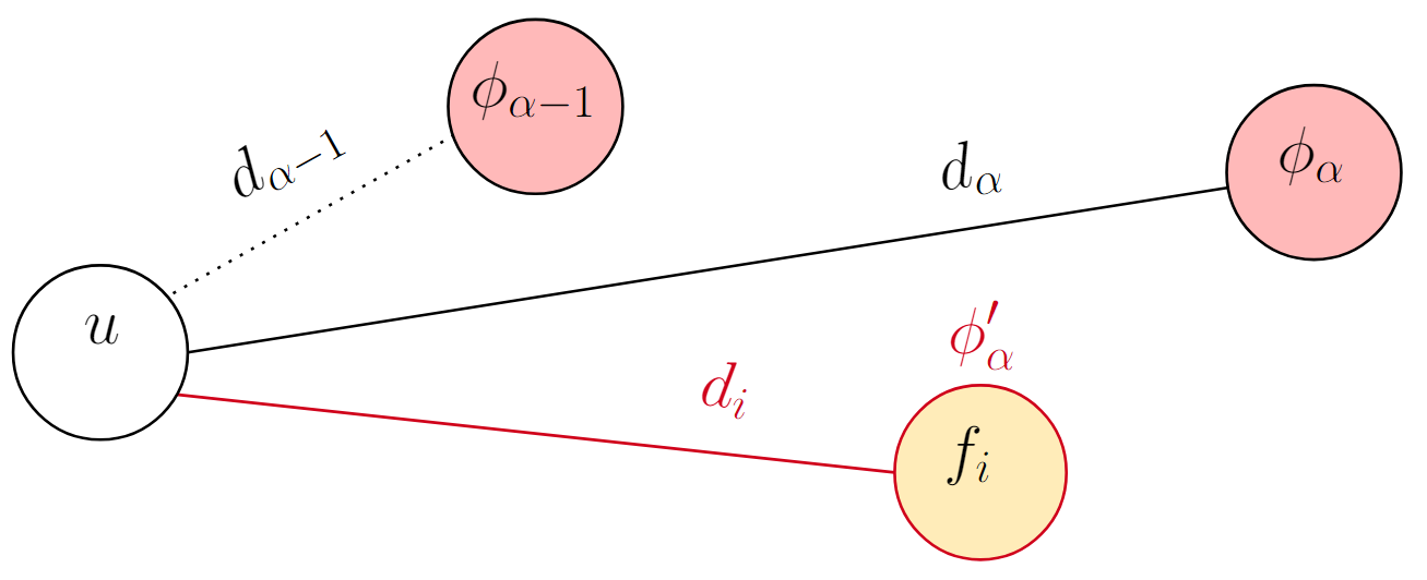
$\phi_\alpha'(u) \gets f_i$
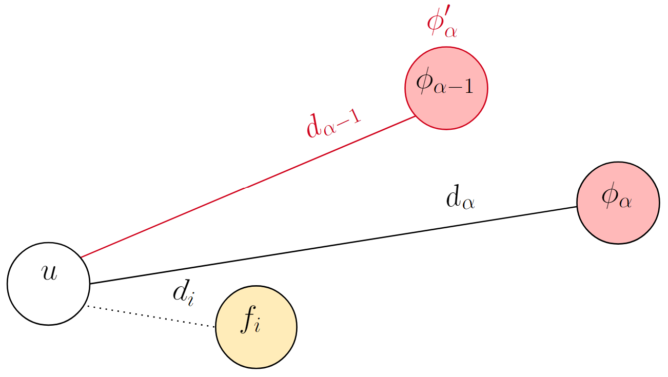
$\phi_\alpha'(u) \gets \phi_{\alpha - 1}(u)$
The two options for the new center when $u$ is attracted to $f_i$ (equation 2).
These observations resulted in modifying FAGI to update the data structures $gain$ and $netloss$ accordingly. However, after applying such modifications, the algorithm did not produce any solutions either. As a consequence, we decided to modify the greedy evaluation step by evaluating the ANPCP’s objective function instead of the PMP’s, and focus on how to calculate the objective function of our problem faster.
Fast Vertex Substitution (FVS)
We found that FAGI was later adapted to solve the PCP, named the fast vertex substitution (FVS), proposed by Mladenović et al. (2003)2. This algorithm also has a worst-case time complexity of $O(mn)$. Now, as mentioned earlier, the ANPCP is a variant of the PCP in which the difference is how the centers are defined. However, the observation that both problems aim to minimize a maximum allowed us to use FVS as a better basis algorithm to adapt for the ANPCP. The key to this adaptation is the use of three data structures that accelerate the search of $f_r$.
In the implementation for the PCP, the new objective function value or radius $x'$, that would result after the interchange, is kept only for users who are attracted by $f_i$, i.e., $f_i$ is closer to them than their center. Besides these new assignments to $f_i$, a new maximum distance $x^*$ could be found among existing assignments. To determine which of these existing connections would remain after a swap, it becomes necessary to store how the radiuses of old centers change when they are considered to be removed or not.
The following conditions apply for users who are not attracted by $f_i$:
-
If a center will be removed ($f_r$), then its users must be reallocated. For each user $u$, its new center would be either its second-closest facility or $f_i$, whichever is the closest to $u$, but incurring a penalty because both options are farther than its old center. The overall penalty is stored in the array $z(\cdot)$, for each center.
-
Otherwise, the radius of that center would not change. This unchanged radius is stored in the array $r(\cdot)$, for each center.
These data structures have size $|S|$ because any open facility can become a center. They get updated by users who are not attracted by $f_i$ and are crucial for the algorithm to decide the most profitable swap, i.e., the best facility to remove given a candidate facility to insert. The pseudocode of this method is described as follows:
Let $x^*(S)$ be the minimum possible objective function value that can result after applying the FVS to the solution $S$, evaluated as the equation 3 below. The formula can be accelerated by keeping track of the two greatest values ($g_1$ and $g_2$ in equation 3) from $r(\cdot)$ while updating the arrays.
$$ \begin{equation} x^*(S) = \min_{f_j \in S}{ \max{ x', z(f_j), \max_{f_l \ne f_j}{ r(f_l) } } } \end{equation} $$
The data structures altogether accelerate the local search by partially evaluating the objective function, using the relations between $f_i$, $U$, and $S$ for every possible swap, stored in $r(\cdot)$, $z(\cdot)$, and $x'$. This stored information allows the algorithm to keep track of multiple maximum distances, without repeating expensive computations, such as a complete revaluation of the objective function.
We tried implementing FVS to solve the ANPCP by applying the equation 2, but without success again. The algorithm kept getting stuck when $\alpha \ge 2$. We observed that the resulting objective function value after an interchange, i.e., a complete modification of the original solution, was unrelated to the information stored in the data structures, meaning that they were not enough to accurately solve the ANPCP. This was likely because it needed to keep track of more relations for this problem than for the PCP.
A detailed evaluation of the FVS on an instance of the PCP proved that the data structures worked correctly as they ended up storing the precise objective function value. This evaluation also helped to better understand the functionality of FVS, making it easier to adapt it for the ANPCP. We propose an adaptation of the FVS to obtain solutions for any value of $\alpha < p$.
In the next subsection, we describe in more detail how we adapted the algorithm to solve the ANPCP.
Alpha Fast Vertex Substitution (A-FVS)
According to the observations explained above, we adapted the FVS for the ANPCP, which from now on we will identify as the Alpha Fast Vertex Substitution (A-FVS), considering first the following modifications:
-
The group of users that is attracted to $f_i$ was divided into two groups and, consequently, into two data structures as well. These two different groups came from the two possible cases for the new center in equation 2. Therefore, a new variable was introduced for the objective function of the second case: $\bar{x'}$. The variable for the first case remained as $x'$.
-
The data structure $z(\cdot)$ was adapted to update all of the $\alpha$-neighbors of every user, and not only its center. The reasoning for this is due to equation 1. Let $A_u$ be, for any user $u$, the set of open facilities closer than or equal to its center, representing the $\alpha$-neighbors of $u$. Note that in the figure below, $\phi_{\alpha + 1}$ is not part of $A_u$, which is shown over purple background.
$$
\begin{gather}
A_u \leftarrow { \phi_k(u) \mid 1 \le k \le \alpha }
\\
\nonumber A_u \subset S, \ u \in U
\end{gather}
$$
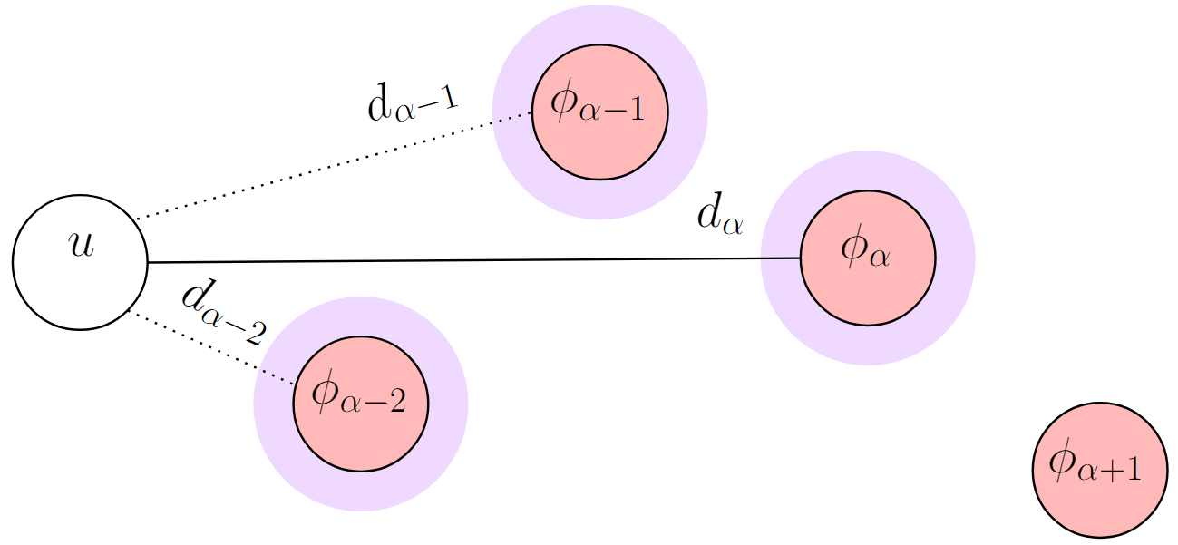
$\alpha$-neighbors of $u$ ($A_u$).
Each one of the $\alpha$-neighbors is an open facility, therefore they can be removed from the solution. In other words, any of them can be selected to be $f_r$.
After evaluating the A-FVS in detail, we observed that the arrays did not accurately store the data between connections of users and centers, and the resulting objective function value was unrelated to them. During this evaluation, the following was noted:
-
The variables for the possible new objective function $x'$ and $\bar{x'}$ could be merged back, just as they were before. It is important to mention that the users still belong to two different groups; however, there is no need to use two different variables, because in any case, the equation applies a $\max$ function on both.
-
The data structure $z(\cdot)$ should be updated for all users, including those who are attracted by $f_i$ because their $\alpha$-neighbors were being considered when finding $f_r$, but these same users were not contributing to the array, so there was no stored information about what would happen to the centers that had any of their $\alpha$-neighbors as $f_r$. This is why the objective function value after a swap and the data in the arrays were mismatched in previous evaluations.
-
As a consequence of the modification to $z(\cdot)$, data structure $r(\cdot)$ should be updated in the same way: for every user and all $\alpha$-neighbors.
With these three observations, all users update and contribute to both arrays $z(\cdot)$ and $r(\cdot)$. This crucial difference from the original FVS is necessary for the ANPCP because both equation 1 and equation 2 are not properties of the PCP, and produced the following additional modifications:
When $f_r$ is an $\alpha$-neighbor
If an $\alpha$-neighbor will be removed ($f_r$), then its users must be reallocated unless they are attracted to $f_i$. In that case, their centers would not change, so the distances to them would remain constant (no penalty), independently of exactly which $\alpha$-neighbor would be removed, and of the exact relative distance from a user $u$ to $f_i$.
Two examples of this case can be visualized below:
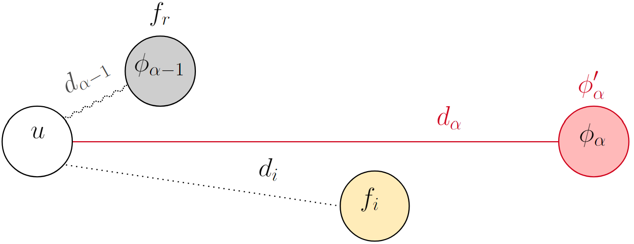
$d_{\alpha - 1} < d_i < d_\alpha$

$d_i < d_{\alpha - 1} < d_\alpha$
If an $\alpha$-neighbor is $f_r$ and $u$ is attracted to $f_i$, its center remains unchanged (no penalty).
However, in the worst case, if they were not attracted to $f_i$, then their new center would be either the $\alpha + 1$ closest facility or $f_i$, whichever is the closest, but still farther than their old center.
Both possibilities are shown below, where the red line is the new assignment of $u$ as well as the penalty of interchanging $f_r$ (the gray $\alpha$-neighbor) with $f_i$. This penalty is stored in the array $z(\cdot)$, for each $\alpha$-neighbor.
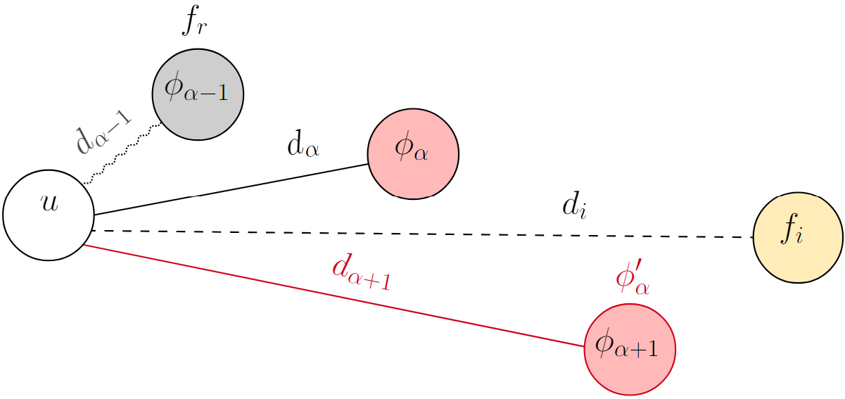
$d_\alpha < d_{\alpha + 1} < d_i$
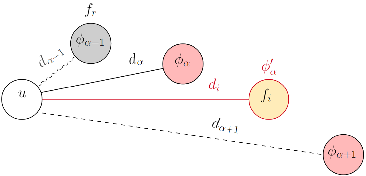
$d_\alpha < d_i < d_{\alpha + 1}$
If an $\alpha$-neighbor is $f_r$ and $u$ is not attracted to $f_i$, its new center will be farther (penalty).
When $f_r$ is not an $\alpha$-neighbor
Otherwise, the radius of that $\alpha$-neighbor would only change if its users are attracted to $f_i$. In that case, their new center would be either the $\alpha - 1$ closest facility or $f_i$, whichever is the farthest, as stated in equation 2 and visualized in its figure, resulting in an improved assignment because this new distance would be shorter.
In the worst case, if they were not attracted to $f_i$, then their center would not change, remaining its radius unchanged. This possible gain is stored in array $r(\cdot)$, for each $\alpha$-neighbor.
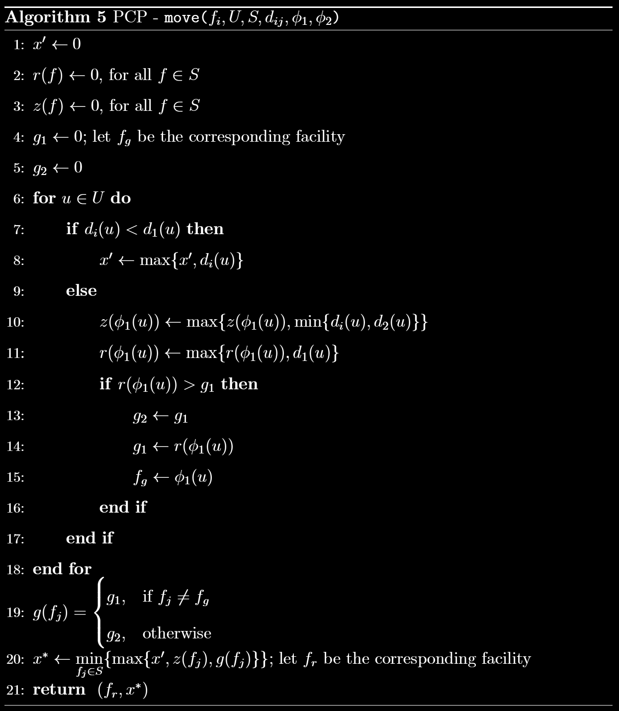
The move procedure
These two final modifications constitute the core step of the A-FVS, which we identify as the move procedure.
The objective of this procedure is, in summary, given a candidate facility to insert, $f_i$, to store the greatest improvement in the objective function in $x'$, and for each $\alpha$-neighbor of every user, to store the greatest penalty of removing it in $z(\cdot)$, and the greatest gain of keeping it in $r(\cdot)$.
Then, it finds the facility that minimizes the maximum of all the distances from the three data structures, and returns both that facility as $f_r$ and that distance as $x^*$.
The formula used in the move procedure to evaluate the resulting objective function after a swap is the same one used in the FVS (equation 3).
This is because the data structures of both algorithms do the same thing: they are just adapted to be updated differently.
This procedure was the first local search modification that yielded an accurate result after evaluating it step by step.
The pseudocode of this procedure is shown below:

Neighborhood reduction
The A-FVS uses an additional acceleration that increasingly reduces the size of the neighborhood $N(S)$ to explore during the iterations, by considering only facilities that would decrease the maximum distance between any user and its center, or “break” the objective function, to be inserted into the solution.
More formally, let the current objective function value $x(S)$ be determined by the distance between a user $u^*$ and its center $f^* = \phi_\alpha(u^*)$, that is, $x(S) = d(u^*, f^*)$. We call critical allocation to the assignment of user-center that determines the objective function, critical user the $u^*$, and critical center the $f^*$.
Note that there will be no improvement of $x$ in $N(S)$ if $f_i$ is farther from $u^*$ than its center ($f^*$) because the critical allocation would not change. Therefore, selecting only facilities closer to $u^*$ than $f^*$ as candidates to insert into $S$ allows us to avoid exploring the whole neighborhood of $S$.
This technique is used in Mladenović et al. (2003)2 for the PCP, and in Sánchez-Oro et al. (2022)3 for the ANPCP as well.
Updates
The concept of the $\alpha$-neighbors is mathematically defined in equation 4 using $\phi_k(u)$, which represents the $k$th closest open facility of a user $u$. This means that the algorithm needs to store what facilities are close to every user and to what degree, which is represented by $k$.
We achieve this by implementing a matrix $M$ of $n$ rows and $m$ columns, where each cell indicates the degree of closeness between a user $u$ and a facility $f$. For each user, the assigned value in $M$ for the open facilities in ${ \phi_k(u) | 1 \le k \le \alpha + 1 }$ is $k$. For the rest of the facilities, including the closed ones, the value is 0. The time complexity to fill $M$ is $O(mn)$ because each cell in the matrix is updated.
This matrix serves as a memory that allows the calculation of the objective function value in $O(pn)$ time. For each user, its center can be found by iterating its row and looking for the column that has $\alpha$ as a value. To avoid visiting the closed facilities, we filter the search by only using the indexes of the open facilities.
This updating step is used in both NI and A-FVS local search algorithms. However, in the NI, the matrix is updated when every swap is considered, while in the A-FVS, it is only updated after a swap is applied to the solution (line 20), reducing the number of times that $M$ is filled.
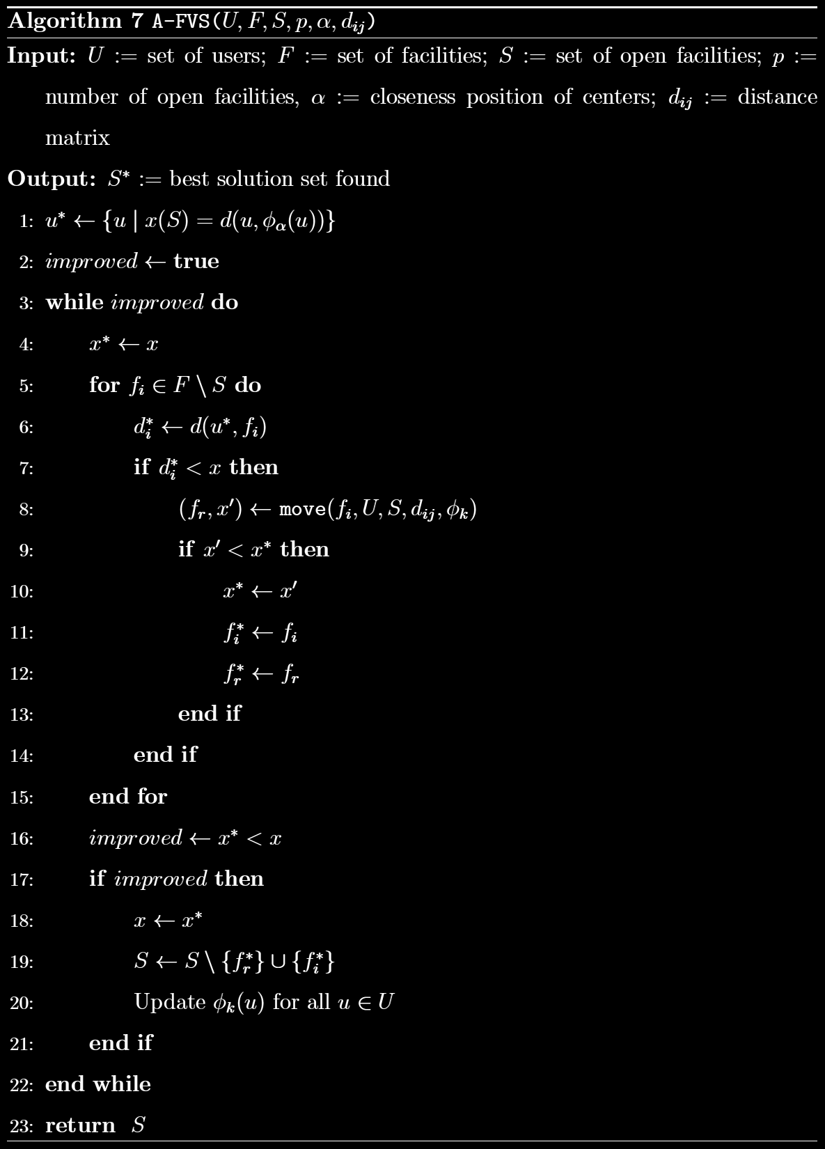
Final algorithm
The complete pseudocode of the A-FVS, including the move that uses the data structures, the technique to reduce the neighborhood, and the updates to the matrix, is shown below:
References
-
R. A. Whitaker. A fast algorithm for the greedy interchange for large-scale clustering and median location problems. INFOR, 21(2):95–108, 1983. ↩︎
-
N. Mladenović, M. Labbé, and P. Hansen. Solving the $p$-center problem with tabu search and variable neighborhood search. Networks, 42(1):48–64, 2003. ↩︎
-
J. Sánchez-Oro, A. D. López-Sánchez, A. G. Hernández-Díaz, and A. Duarte. GRASP with strategic oscillation for the $\alpha$-neighbor $p$-center problem. European Journal of Operational Research, 2022. ↩︎